The 10 Basic Excel Formulas Everyone Needs to Know

Learn how to add arithmetic, string, time series, and complex formulas in Microsoft Excel.

What is an Excel Formula?

Microsoft Excel is a popular tool for managing data and performing data analysis. It is used for generating analytical reports, business insights, and storing operational records. To perform simple calculations or analyses on data, we need Excel formulas.

Even simple Excel formulas allow us to manipulate string, number, and date data fields. Furthermore, you can use if-else statements, find and replace, mathematics and trigonometry, finance, logical, and engineering formulas.

Unlike programming languages, you will be writing the formula name and arguments. That’s it, nothing complex. You can also use Excel-assisted user interference to add formulas.

Why Are Excel Formulas Important?

Excel formulas are essential for several reasons:

1. Efficiency: They automate repetitive tasks, saving time and reducing manual errors.

2. Data analysis: Excel's range of formulas enables sophisticated data analysis, crucial for informed decision-making.

3. Accuracy: Formulas ensure consistent and accurate results, essential in fields like finance and accounting.

4. Data manipulation: They allow for efficient sorting, filtering, and manipulation of large datasets.

5. Accessibility: Excel provides a user-friendly platform, making complex data analysis accessible to non-technical users.

6. Versatility: Widely used across various industries, proficiency in Excel formulas enhances employability and career advancement.

7. Customization: Excel offers customizable formula options to meet specific data handling needs.

In essence, Excel formulas are a foundational tool for effective data management, analysis, and decision-making.

How to Use Excel Formulas

Adding the Excel formula is relatively easy. It will come to you naturally if you are familiar with any business intelligence software.  

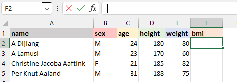
The most effective and fast way to use formulas is by adding them manually. In the example below, we are calculating the BMI (Body Mass Index) of the athletes shown in the table.

BMI = weight (KG)/ (Height (m))2 

1. Choose the cell for the resulting output. You can use the mouse to select the cell or use the arrow key to navigate. 

2. Type “=” in the cell. The equal sign will appear in the cell and formula bar. 

3. Type the address of the cell that we want to use for our calculation. In our case, it is E2 (weight/KG).

4. Add divide sign “/”

5. To convert height from centimeters to a meter, we will divide the D2 by 100.

6. Take the squared “^2” of the height and press Enter. 

Note: To get the address of any cell, you need to look at the column name (A, B, C, … ) and combine it with a row number (1, 2, 3, …). For example, A2, B5, and C12   

That’s it; we have successfully calculated the BMI of A Dijiang.

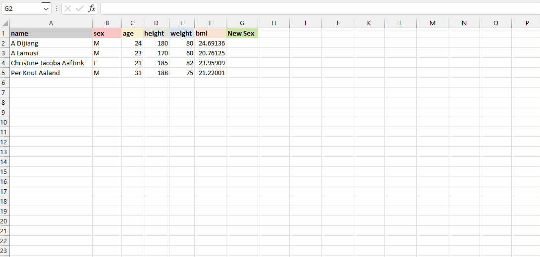
We can also add the Excel formula by using assisted GUI. It is simple. 

In the example below, we will be using GUI to add an IF formula to convert ‘M’ to ‘Male’ and ‘F’ to Female.

1. Click on the fx button next to the formula bar.

2. It will pop up in the window with the most used function.

3. You can either search for the specific formula or select the formula by scrolling. In our case, we will be specifying the IF formula. 

4. Add the logic B2=’M” into the logical_test argument.

5. Add “Male” in value_if_true argument and “Female” in value_if_false argument. 

The formula works similarly to the if else statement. If the logical_test statement is TRUE, the formula will return “Male” otherwise “Female.”

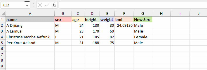
How to insert formulas in excel for an entire column

We have learned to add the formula to a single row. Now, we will learn to apply the same formula to the entire column. 

There are multiple ways to add formulas: 

• Dragging down the fill handle: when you select the cell, you will see the small green box at the bottom right. It is called a fill handle. Click and hold the fill handle and drag it down to the last row. It is commonly used to apply formulas to selected rows. 

• Double click the fill handle: select the cell with the formula and double click the fill handle. Within seconds it will apply the formula to the entire column. 

• Shortcut: select the cell with the formula and the empty cells below it. Press CTRL + D to apply the formula. Make sure you are not selecting anything above the formula cell. 

• Copy-pasting: copy the cell with the formula (CTRL + C), select the empty rows in a column, and paste it (CTRL + V). Make sure you are not using a fill handle to select the rows. 

The visual representation below shows all the ways we can apply the formula to multiple cells. 

Basic Formulas in Excel 

Now that we know how to use Excel formulas, it’s time to learn about 15 basic Excel formulas on a small subset of the Olympics dataset from DataCamp. To keep things simple, we will mainly use the name, sex, age, height, and weight columns of four athletes' records. 

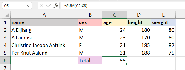
1. SUM

The SUM() formula performs addition on selected cells. It works on cells containing numerical values and requires two or more cells.  

In our case, we will be applying the SUM formula to a range of cells from C2 to C5 and storing the result on C6. It will add 24, 23, 21, and 31. You can also apply this formula to multiple columns.

=SUM(C2:C5)

This code is written in Microsoft Excel formula language.

• It calculates the sum of the values in cells C2 to C5 and returns the result.

• The equal sign at the beginning of the formula indicates that it is a formula and not just a regular text entry.

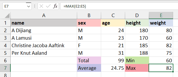
2. MIN and MAX

The MIN() formula requires a range of cells, and it returns the minimum value. For example, we want to display the minimum weight among all athletes on the E6 cell. The MIN formula will search for the minimum value and show 60.

=MIN(E2:E5)

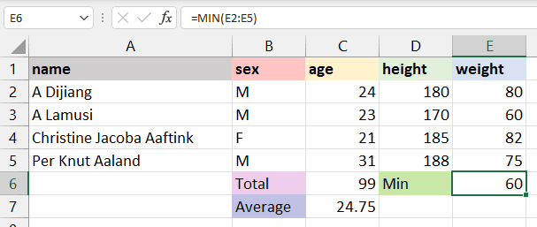
This code is written in Microsoft Excel formula language.

• The formula =MAX(E2:E5) finds the maximum value in the range of cells E2 to E5.

• It returns the highest value in that range.

• For example, if the values in cells E2 to E5 are 5, 10, 3, and 8, then the formula =MAX(E2:E5) will return 10, which is the highest value in that range.

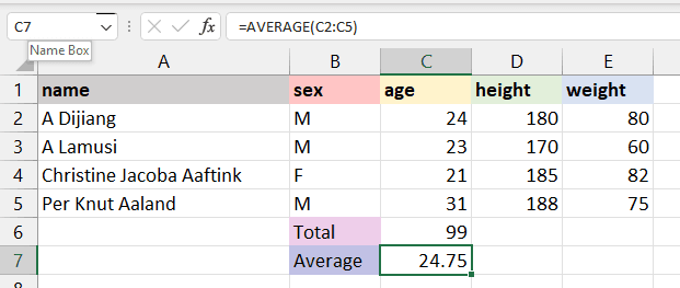
3. AVERAGE

The AVERAGE() formula calculates the average of selected cells. You can provide a range of cells (C2:C5) or select individual cells (C2, C3, C5).

To calculate the average of athletes, we will select the age column, apply the average formula, and return the result to the C7 cell. It will sum up the total values in the selected cells and divide them by 4.

=AVERAGE(C2:C5) 

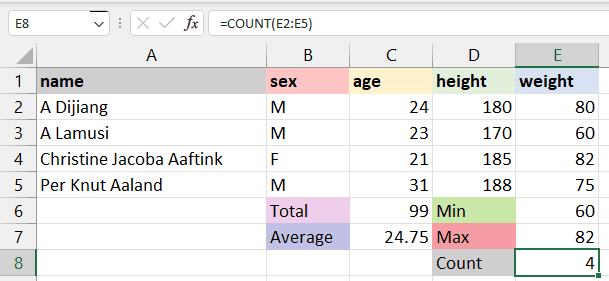
4. COUNT

The COUNT() formula counts the total number of selected cells. It will not count the blank cells and different data formats other than numeric. 

We will count the total number of athlete weights, and it will return 4, as we don’t have missing values or strings. 

=COUNT(E2:E5)

To count all types of cells (date-time, string, numerical), you need to use the COUNTA() formula. 

The COUNTA formula does not count missing values. For blank cells, use COUNTBLANK().

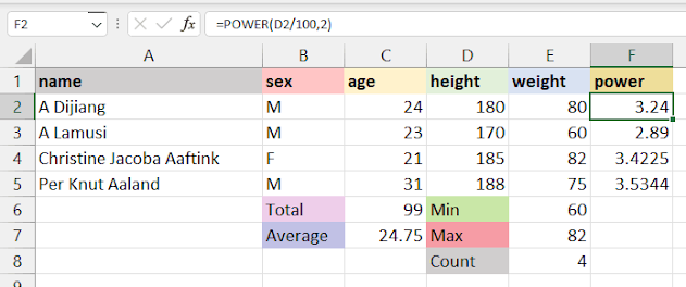
5. POWER

In the beginning, we learned to add power using “^”, which is not an efficient way of applying power to a cell. Instead, we recommended using the POWER() formula to square, cube, or apply any raise to power to your cell. 

In our case, we have divided D2 by 100 to get height in meters and squared it by using the POWER formula with the second argument as 2.   

=POWER(D2/100,2)

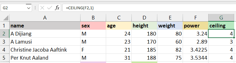
6. CEILING and FLOOR

The CEILING() formula rounds a number up to the nearest given multiple. In our case, we will round 3.24 up to a multiple of 1 and get 4. If the multiple is 5, it will round up the number 3.24 to 5.  

=CEILING(F2,1)

The FLOOR() rounds a number down to the nearest given multiple. As we can see in the image below, instead of converting 3.24 to 4, it has rounded the number to 3. 

=FLOOR(F2,1)

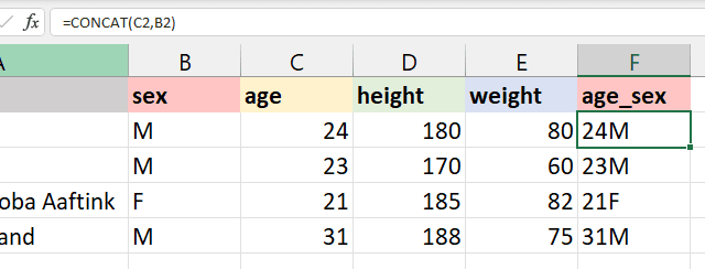
7. CONCAT

The CONCAT() Excel formula joins or merges multiple strings or cells with strings into one. For example, if we want to join the age and sex of the athletes, we will use CONCAT. The formula will automatically convert a numeric value from age to string and combine it. 

“24”+“M” = “24M”

=CONCAT(C2,B2)

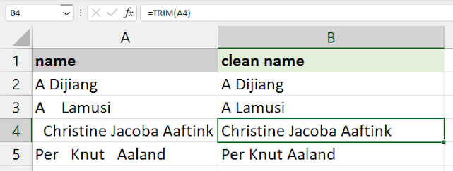
8. TRIM

TRIM is used to remove extra spaces from the start, middle, and end. It is commonly used to identify duplicate values in cells, and for some reason, extra space makes it unique.  

For example:

1. There are extra two spaces at A3 “A   Lamusi”, and it has been successfully removed by TRIM.

2. At A4 “ Christie Jacoba Aaftink”, there is extra space at the start, and without writing any complex formula, the TRIM has removed it. 

=TRIM(A4)

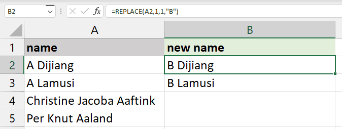
9. REPLACE and SUBSTITUTE

REPLACE is used for replacing part of the string with a new string.

REPLACE(old_text, start_num, num_chars, new_text) 

• old_text is the original text or cell containing the text.

• start_num is the index position that you want to start replacing the character. 

• num_chars refers to the number of characters you want to replace.

• new_text indicates the new text that you want to replace with old text. 

For example, we will change A Dijiang with B Dijiang by providing the positing of character, which is 1, the number of characters that we want to replace, which is also 1, and the new character “B”. 

=REPLACE(A2,1,1,"B")

The SUBSTITUTE formula is similar to REPLACE. Instead of providing the location of a character or the number of characters, we will only provide old text and new text. 

SUBSTITUTE(text, old_text, new_text, [instance_num])

In our case, we are replacing "Jacoba" with "Rahim" to display the result on A4 cell “Christine Rahim Aaftink.”

This formula is quite useful as it does not change the text without “Jacoba” as shown below in cell A5, “Per Knut Aaland.” Whereas, REPLACE will replace the text every time. 

=SUBSTITUTE(A4,"Jacoba","Rahim")

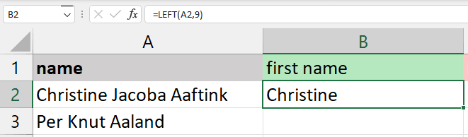
10. LEFT, RIGHT, and MID

The LEFT returns the number of characters from the start of the string or text. 

For example, to display the first name from the text “Christine Jacoba Aaftink”, you will use LEFT with 9  numbers of characters. As a result, it will show the first nine characters; “Christine.”

=LEFT(A2,9)

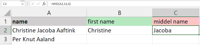
The MID formula requires starting position and length to extract the characters from the middle. 

For example, if you want to display a middle name, you will start with “J” which is at the 11th position, and 6 for the length of the middle name “Jacoba”.

=MID(A2,11,6)

The RIGHT will return the number of characters from the end. You just need to provide a number of characters. 

For example, to display the last name “Aaftink,” we will use RIGHT with seven characters.